Quantum Nonlocality, and Bells Theorem has been conjured up on ocassion to explain psi phenomena. My evolving project may have relevance here. http://www.p2pfoundation.net/Multi-Dimensional_Science
RS.
From Wikipedia, the free encyclopedia
Quantum Nonlocality
Generally, quantum nonlocality is the phenomenon by which microscopic objects seem to interact instantaneously (or nearly instantaneously) at a distance without any apparent intervening force. The phenomenon violates the common notion that an object may be directly influenced only by its immediate surroundings (the principle of locality).
This would seem to allow for faster-than-light communication.[1] However, because the distant connections are statistical probabilities involving measurements that require subluminal channels for confirmation (see examples below), as of 2012[update] faster-than-light communication has not been observed and therefore quantum nonlocality is still compatible with special relativity's speed limit.
As of 2012[update], quantum nonlocality has only been observed with quantum entanglement, which occurs when particles such as photons, electrons, and some larger objects,[2][3][4][5] interact physically and then become separated. The interaction is such that the quantum state of one member of the entangled pair is correlated to the state of the other member of the pair. When a property of one entangled member is measured and definitely known, the property of the other member then becomes entirely predictable (i.e., it instantly changes from being indefinite to definite).[6] Even though entanglement is compatible with relativity, it prompts more fundamental discussions concerning quantum theory. For example, it has been proposed[7] that quantum mechanics cannot be more non-local without violating the Heisenberg uncertainty principle. A more general nonlocality beyond quantum entanglement, yet retaining compatibility with relativity, is an active field of theoretical investigation and has yet to be observed.
The experimental evidence of quantum nonlocality has resulted in the general rejection of a previous theory known as local hidden variable theory in which distant events were assumed to have no instantaneous (or at least faster-than-light) effect on local ones. However, whether quantum entanglement counts as action-at-a-distance hinges on the nature of the wave function and decoherence, issues over which as of 2012[update] there is still considerable debate among scientists and philosophers.[8] Non-standard interpretations of quantum mechanics have varied in their response to quantum nonlocality. These include the Bohm interpretation,[9] counterfactual definiteness, the consciousness causes collapse theory, and the EPR paradox thought experiment.
Quantum nonlocality is of much interest because of potential practical applications, such as quantum computing and faster-than-light communication.
More realistically, suppose that the four events occur with (conditional) probabilities P(b0|A0), P(b1|A0) = 1 - P(b0|A0), P(b0|A1) and P(b1|A1) = 1 - P(b0|A1). Here P(b0|A0) is the probability that Bob's b0 lamp lit up, given that Alice pushed the button A0. We can still rigorize the notion that A has an influence on B in this setting: if P(b0|A0) differs from P(b0|A1) then Alice's choice of button still affects the probabilistic outcome on Bob's side, and it is still possible for Alice to send Bob messages with low probability of error. For example, if P(b0|A0) = and P(b0|A1) =
  , then after 100 runs of the experiment in which Alice pushed the same button, Bob can tell with high probability which button it was by looking at how often b0 occurred.
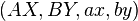
Here is a more complicated scenario: Alice pushes one of two buttons, A0 and A1, and Bob also pushes one of two buttons, B0 and B1. Alice observes one of two outcomes, a0 and a1, and Bob also observes one of two outcomes, b0 and b1. There are 24 = 16 possible combinations of these 4 events:
 denotes addition modulo 2.
Then if A1 and B1 are both pressed ( (A1,B1) chosen) the outcomes are perfectly anticorrelated, either (a0,b1) or (a1,b0), with an equal probability for both occurrences. In all other cases the two outcomes are perfectly correlated (either (a0,b0) or (a1,b1), again, equiprobably.
Do these outcomes imply that some influence exists (A on B, or B on A), or not? The question is important, since the answer depends on our fundamental assumptions about how mathematical theories describe physical reality.
On the one hand, Alice cannot send a message to Bob, using her buttons A0, A1 and his indicators b0, b1 (nor Bob to Alice). In this sense there is no influence of A on B, or of B on A, since it is easily checked that P(bx|A0) = P(bx|A1) for both x = 0 and x = 1 in the above example. That is to say, this particular set of probabilities is non-signalling.
On the other hand, it is provably impossible for two separated parties to simulate this outcome without any kind of interaction or communication between them.[10] Thorough logical analysis reveals that the above outcome can only occur if there is some direct influence between A and B, if we assume local realism and, arguably, counterfactual definiteness. These fundamental assumptions, deeply rooted in our physical intuition, are incompatible with quantum theory. Different interpretations of quantum mechanics reject different parts of local realism and/or counterfactual definiteness (for detail, see Principle of locality). A classical definition of nonlocality, i.e. direct influence of one object on another, distant object, normally takes local realism and counterfactual definiteness for granted.
Bell formalized the idea of a hidden variable by introducing the parameter λ to locally characterize measurement results on each system:[19] "It is a matter of indifference... whether λ denotes a single variable or a set... and whether the variables are discrete or continuous". However, it is equivalent (and more intuitive) to think of λ as a local "strategy" that occurs with some probability ρ( ) when an entangled pair of states is created. EPR's criteria of local separability then stipulates that each local strategy defines independent distributions for the outcome probabilities if Alice measures in direction A and Bob measures in direction B:
 denotes the probability of Alice getting the outcome a given λ, and that she measured A.
Suppose that λ can take values from some set , where 1 ≤ i ≤ k. If each has an associated probability ρ() of being selected (such that the probabilities sum to unity) we can average over this distribution to obtain a formula for the joint probability of each measurement result:
 or
or  , and Bob chooses from
  or
or  , the CHSH value for this joint probability distribution is defined as:
 and the discussion in the above example. The CHSH value
  includes a negative contribution of the correlator whenever and are chosen (
 when
when  ), and a positive contribution in all other cases (
 ≠
≠ when
when  ). If the joint probability distribution can be described with local strategies as above, it can be shown that the correlation function always obeys the following CHSH inequality[13]:
 such that
  . Experimentalists such as Aspect have verified the quantum violation of the CHSH inequality,[21] as well as other formulations of Bell's inequality, to invalidate the local hidden variables hypothesis and confirm that reality is indeed nonlocal in the EPR sense.
 , even if we exploit measurements of entangled particles.[22] The question remained whether this was the maximum CHSH value that can be attained without explicitly allowing instantaneous signaling. In 1994 two physicists, Sandu Popescu and Daniel Rohrlich, formulated an explicit set of non-signalling correlated measurements that give
  : the algebraic maximum.[10] This demonstrated that there are apparently reasonable theories of parts of Nature that drastically violate the predictions of quantum theory. The attempt to understand what uniquely identifies quantum theory from such general theories motivated an abstraction from physical measurements of nonlocality, to the study of nonlocal boxes.[23]
Nonlocal boxes generalize the concept of experimentalists making joint measurements from separate locations. As in the discussion above, the choice of measurement is encoded by the input to the box. A two-party nonlocal box takes an input A from Alice and an input B from Bob, and outputs two values a and b for Alice and Bob respectively and separately, where a, b, A and B take values from some finite alphabet (normally ). The box is characterized by the probability of outputting pair a, b, given the inputs A, B. This probability is denoted
  and obeys the normal probabilistic conditions of positivity and normalisation:[23]
 and
and  describe single input/output probabilities at Alice's or Bob's system alone, and the value of is chosen at random according to some fixed probability distribution given by
  . Intuitively, corresponds to a hidden variable, or to a shared randomness between Alice and Bob. If a box violates this condition, it is explicitly nonlocal. However, the study of nonlocal boxes often also encapsulates local boxes.
The set of nonlocal boxes most commonly studied are the so-called non-signalling boxes,[23] for which neither Alice nor Bob can signal their choice of input to the other. Physically, this is a reasonable restriction: setting the input is physically analogous to making a measurement, which should effectively provide a result immediately. Since there may be a large spatial separation between the parties, signalling to Bob would potentially require considerable time to elapse between measurement and result, which is a physically unrealistic scenario.
The non-signalling requirement imposes further conditions on the joint probability, in that the probability of a particular output a or b should depend only on its associated input. This allows for the notion of a reduced or marginal probability on both Alice and Bob's measurements, and is formalised by the conditions:
with probabilities ) to produce another box that also exists within the polytope.
Local boxes are clearly non-signalling, however nonlocal boxes may or may not be non-signalling. Since this polytope contains all possible non-signalling boxes of a given number of inputs and outputs, it has as subsets both local boxes and those boxes which can achieve Tsirelson’s bound in accord with quantum mechanical correlations. Indeed, the set of local boxes form a convex sub-polytope of the non-signalling polytope.
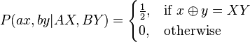
Popescu and Rohrlich’s maximum algebraic violation of the CHSH inequality can be reached by a non-signalling box, referred to as a standard PR box after these authors, with joint probability given by:
 denotes addition modulo two.[25]
Various attempts have been made to explain why Nature does not allow for stronger nonlocality than quantum theory permits. For example, in a recent publication it was found that quantum mechanics cannot be more nonlocal without violating the Heisenberg uncertainty principle.[26] Strikingly, it has been discovered that if PR boxes did exist, any distributed computation could be performed with only one bit of communication.[27] An even stronger result is that for any nonlocal box theory which violates Tsirelson's bound, there cannot be a sensible measure of mutual information between pairs of systems.[28] This suggests a deep link between nonlocality and the information-theoretic properties of quantum mechanics.
 , but can always be described using local hidden variables.[24] On the other hand, reasonably simple examples of Bell inequalities have been found for which the quantum state giving the largest violation is never a maximally entangled state, showing that entanglement is, in some sense, not even proportional to nonlocality. [29] [30] [31]
In short, entanglement of a two-party state is necessary but not sufficient for that state to be nonlocal. It is important to recognise that entanglement is more commonly viewed as an algebraic concept, noted for being a precedent to nonlocality as well as quantum teleportation and superdense coding, whereas nonlocality is interpreted according to experimental statistics and is much more involved with the foundations and interpretations of quantum mechanics.
This would seem to allow for faster-than-light communication.[1] However, because the distant connections are statistical probabilities involving measurements that require subluminal channels for confirmation (see examples below), as of 2012[update] faster-than-light communication has not been observed and therefore quantum nonlocality is still compatible with special relativity's speed limit.
As of 2012[update], quantum nonlocality has only been observed with quantum entanglement, which occurs when particles such as photons, electrons, and some larger objects,[2][3][4][5] interact physically and then become separated. The interaction is such that the quantum state of one member of the entangled pair is correlated to the state of the other member of the pair. When a property of one entangled member is measured and definitely known, the property of the other member then becomes entirely predictable (i.e., it instantly changes from being indefinite to definite).[6] Even though entanglement is compatible with relativity, it prompts more fundamental discussions concerning quantum theory. For example, it has been proposed[7] that quantum mechanics cannot be more non-local without violating the Heisenberg uncertainty principle. A more general nonlocality beyond quantum entanglement, yet retaining compatibility with relativity, is an active field of theoretical investigation and has yet to be observed.
The experimental evidence of quantum nonlocality has resulted in the general rejection of a previous theory known as local hidden variable theory in which distant events were assumed to have no instantaneous (or at least faster-than-light) effect on local ones. However, whether quantum entanglement counts as action-at-a-distance hinges on the nature of the wave function and decoherence, issues over which as of 2012[update] there is still considerable debate among scientists and philosophers.[8] Non-standard interpretations of quantum mechanics have varied in their response to quantum nonlocality. These include the Bohm interpretation,[9] counterfactual definiteness, the consciousness causes collapse theory, and the EPR paradox thought experiment.
Quantum nonlocality is of much interest because of potential practical applications, such as quantum computing and faster-than-light communication.
Contents |
[edit] Example
Imagine two experimentalists, Alice and Bob, situated in separate laboratories. They conduct a simple experiment in which Alice chooses and pushes one of two buttons, A0 and A1, on her apparatus, and Bob observes on his apparatus one of two indicating lamps, b0 and b1, lighting. In this case there are four possible events that could occur in the experiment: (A0,b0), (A0,b1), (A1,b0) and (A1,b1). Suppose that after many runs of the experiment, only the events (A0,b0) and (A1,b1) occur; this is good evidence that A has an influence on B. Indeed, Alice could easily send messages to Bob by encoding those messages into sequences of 0's and 1's, and causing the b0 or b1 lamp to light up respectively.More realistically, suppose that the four events occur with (conditional) probabilities P(b0|A0), P(b1|A0) = 1 - P(b0|A0), P(b0|A1) and P(b1|A1) = 1 - P(b0|A1). Here P(b0|A0) is the probability that Bob's b0 lamp lit up, given that Alice pushed the button A0. We can still rigorize the notion that A has an influence on B in this setting: if P(b0|A0) differs from P(b0|A1) then Alice's choice of button still affects the probabilistic outcome on Bob's side, and it is still possible for Alice to send Bob messages with low probability of error. For example, if P(b0|A0) =
and P(b0|A1) = , then after 100 runs of the experiment in which Alice pushed the same button, Bob can tell with high probability which button it was by looking at how often b0 occurred.Here is a more complicated scenario: Alice pushes one of two buttons, A0 and A1, and Bob also pushes one of two buttons, B0 and B1. Alice observes one of two outcomes, a0 and a1, and Bob also observes one of two outcomes, b0 and b1. There are 24 = 16 possible combinations of these 4 events:
 denotes addition modulo 2.
Then if A1 and B1 are both pressed ( (A1,B1) chosen) the outcomes are perfectly anticorrelated, either (a0,b1) or (a1,b0), with an equal probability for both occurrences. In all other cases the two outcomes are perfectly correlated (either (a0,b0) or (a1,b1), again, equiprobably.
Do these outcomes imply that some influence exists (A on B, or B on A), or not? The question is important, since the answer depends on our fundamental assumptions about how mathematical theories describe physical reality.
On the one hand, Alice cannot send a message to Bob, using her buttons A0, A1 and his indicators b0, b1 (nor Bob to Alice). In this sense there is no influence of A on B, or of B on A, since it is easily checked that P(bx|A0) = P(bx|A1) for both x = 0 and x = 1 in the above example. That is to say, this particular set of probabilities is non-signalling.
On the other hand, it is provably impossible for two separated parties to simulate this outcome without any kind of interaction or communication between them.[10] Thorough logical analysis reveals that the above outcome can only occur if there is some direct influence between A and B, if we assume local realism and, arguably, counterfactual definiteness. These fundamental assumptions, deeply rooted in our physical intuition, are incompatible with quantum theory. Different interpretations of quantum mechanics reject different parts of local realism and/or counterfactual definiteness (for detail, see Principle of locality). A classical definition of nonlocality, i.e. direct influence of one object on another, distant object, normally takes local realism and counterfactual definiteness for granted.
[edit] History
[edit] Einstein, Podolsky and Rosen
Main article: EPR Paradox
In 1935, Einstein, Podolsky and Rosen published a thought experiment[11] with which they hoped to expose the incompleteness of the Copenhagen interpretation of quantum mechanics in relation to the violation of realism and local causality at the microscopic scale that it described. David Bohm later modified the original EPR thought experiment,[12] simplifying the mathematics and highlighting assumptions like locality (which Einstein et al had tacitly assumed). In Bohm's version of the experiment, a spin-zero particle decays into two spin-half particles such that there is no interaction between the two particles after decay. The quantum state of the two particles prior to measurement can be written as[13]

- While we have thus shown that the wave function does not provide a complete description of the physical reality, we left open the question of whether or not such a description exists. We believe, however, that such a theory is possible.
[edit] Demonstration
See also: Bell test experiments
In 1964 John Bell showed that such local hidden variables could never reproduce the statistical outcomes of individual measurements, as predicted by quantum theory.[19] Bell showed that a local hidden variable hypothesis leads to restrictions on the strength of correlations of measurement results. If the Bell inequalities are violated experimentally as predicted by quantum mechanics, then reality cannot be described by such local hidden variables and the mystery of quantum nonlocal causation remains. According to Bell:[19]- This [grossly nonlocal structure] is characteristic... of any such theory which reproduces exactly the quantum mechanical predictions.
Bell formalized the idea of a hidden variable by introducing the parameter λ to locally characterize measurement results on each system:[19] "It is a matter of indifference... whether λ denotes a single variable or a set... and whether the variables are discrete or continuous". However, it is equivalent (and more intuitive) to think of λ as a local "strategy" that occurs with some probability ρ(
) when an entangled pair of states is created. EPR's criteria of local separability then stipulates that each local strategy defines independent distributions for the outcome probabilities if Alice measures in direction A and Bob measures in direction B: denotes the probability of Alice getting the outcome a given λ, and that she measured A.
Suppose that λ can take values from some set
, where 1 ≤ i ≤ k. If each has an associated probability ρ() of being selected (such that the probabilities sum to unity) we can average over this distribution to obtain a formula for the joint probability of each measurement result: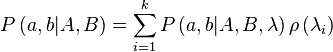
 or , and Bob chooses from or , the CHSH value for this joint probability distribution is defined as:
 and the discussion in the above example. The CHSH value includes a negative contribution of the correlator whenever and are chosen ( when ), and a positive contribution in all other cases (≠ when ). If the joint probability distribution can be described with local strategies as above, it can be shown that the correlation function always obeys the following CHSH inequality[13]:
 such that . Experimentalists such as Aspect have verified the quantum violation of the CHSH inequality,[21] as well as other formulations of Bell's inequality, to invalidate the local hidden variables hypothesis and confirm that reality is indeed nonlocal in the EPR sense.
[edit] Superquantum nonlocality
Whilst the CHSH inequality gives restrictions on the CHSH value attainable by local hidden variable theories, the rules of quantum theory do not allow us to violate Tsirelson's bound of, even if we exploit measurements of entangled particles.[22] The question remained whether this was the maximum CHSH value that can be attained without explicitly allowing instantaneous signaling. In 1994 two physicists, Sandu Popescu and Daniel Rohrlich, formulated an explicit set of non-signalling correlated measurements that give : the algebraic maximum.[10] This demonstrated that there are apparently reasonable theories of parts of Nature that drastically violate the predictions of quantum theory. The attempt to understand what uniquely identifies quantum theory from such general theories motivated an abstraction from physical measurements of nonlocality, to the study of nonlocal boxes.[23]Nonlocal boxes generalize the concept of experimentalists making joint measurements from separate locations. As in the discussion above, the choice of measurement is encoded by the input to the box. A two-party nonlocal box takes an input A from Alice and an input B from Bob, and outputs two values a and b for Alice and Bob respectively and separately, where a, b, A and B take values from some finite alphabet (normally
). The box is characterized by the probability of outputting pair a, b, given the inputs A, B. This probability is denoted and obeys the normal probabilistic conditions of positivity and normalisation:[23]

 and describe single input/output probabilities at Alice's or Bob's system alone, and the value of is chosen at random according to some fixed probability distribution given by . Intuitively, corresponds to a hidden variable, or to a shared randomness between Alice and Bob. If a box violates this condition, it is explicitly nonlocal. However, the study of nonlocal boxes often also encapsulates local boxes.
The set of nonlocal boxes most commonly studied are the so-called non-signalling boxes,[23] for which neither Alice nor Bob can signal their choice of input to the other. Physically, this is a reasonable restriction: setting the input is physically analogous to making a measurement, which should effectively provide a result immediately. Since there may be a large spatial separation between the parties, signalling to Bob would potentially require considerable time to elapse between measurement and result, which is a physically unrealistic scenario.
The non-signalling requirement imposes further conditions on the joint probability, in that the probability of a particular output a or b should depend only on its associated input. This allows for the notion of a reduced or marginal probability on both Alice and Bob's measurements, and is formalised by the conditions:

 with probabilities ) to produce another box that also exists within the polytope.
Local boxes are clearly non-signalling, however nonlocal boxes may or may not be non-signalling. Since this polytope contains all possible non-signalling boxes of a given number of inputs and outputs, it has as subsets both local boxes and those boxes which can achieve Tsirelson’s bound in accord with quantum mechanical correlations. Indeed, the set of local boxes form a convex sub-polytope of the non-signalling polytope.
Popescu and Rohrlich’s maximum algebraic violation of the CHSH inequality can be reached by a non-signalling box, referred to as a standard PR box after these authors, with joint probability given by:
 denotes addition modulo two.[25]
Various attempts have been made to explain why Nature does not allow for stronger nonlocality than quantum theory permits. For example, in a recent publication it was found that quantum mechanics cannot be more nonlocal without violating the Heisenberg uncertainty principle.[26] Strikingly, it has been discovered that if PR boxes did exist, any distributed computation could be performed with only one bit of communication.[27] An even stronger result is that for any nonlocal box theory which violates Tsirelson's bound, there cannot be a sensible measure of mutual information between pairs of systems.[28] This suggests a deep link between nonlocality and the information-theoretic properties of quantum mechanics.
[edit] Nonlocality vs entanglement
See also: Quantum entanglement
In the media and popular science, quantum nonlocality is often portrayed as being equivalent to entanglement. While it is true that a bipartite quantum state must be entangled in order for it to produce nonlocal correlations, there exist entangled states which do not produce such correlations. A well-known example of this is the Werner state that is entangled for certain values of , but can always be described using local hidden variables.[24] On the other hand, reasonably simple examples of Bell inequalities have been found for which the quantum state giving the largest violation is never a maximally entangled state, showing that entanglement is, in some sense, not even proportional to nonlocality. [29] [30] [31]In short, entanglement of a two-party state is necessary but not sufficient for that state to be nonlocal. It is important to recognise that entanglement is more commonly viewed as an algebraic concept, noted for being a precedent to nonlocality as well as quantum teleportation and superdense coding, whereas nonlocality is interpreted according to experimental statistics and is much more involved with the foundations and interpretations of quantum mechanics.
[edit] See also
[edit] References
- ^ Ghirardi, G.C.; Rimini, A. and Weber, T. (March 1980). "A general argument against superluminal transmission through the quantum mechanical measurement process". Lettere Al Nuovo Cimento 27 (10): 293–298. doi:10.1007/BF02817189.
- ^ Nature: Wave–particle duality of C60 molecules, 14 October 1999. Abstract, subscription needed for full text
- ^ Olaf Nairz, Markus Arndt, and Anton Zeilinger, "Quantum interference experiments with large molecules", American Journal of Physics, 71 (April 2003) 319-325.
- ^ K. C. Lee, M. R. Sprague, B. J. Sussman, J. Nunn, N. K. Langford, X.-M. Jin, T. Champion, P. Michelberger, K. F. Reim, D. England, D. Jaksch, I. A. Walmsley (2 December 2011). "Entangling macroscopic diamonds at room temperature". Science 334 (6060): 1253–1256. doi:10.1126/science.1211914. http://www.sciencemag.org/content/334/6060/1253.full. Lay summary.
- ^ sciencemag.org, supplementary materials
- ^ "Wave functions could describe combinations of different states, so-called superpositions. For example, an electron could be in a superposition of several different locations", from Max Tegmark; John Archibald Wheeler (2001). "100 Years of the Quantum". Sci.Am.:,; Spektrum Wiss. Dossier N1:6-14 284 (2003): 68–75. arXiv:quant-ph/0101077.
- ^ If quantum mechanics were more non-local it would violate the uncertainty principle - http://arxiv.org/PS_cache/arxiv/pdf/1004/1004.2507v1.pdf
- ^ Berkovitz, J. "Action at a Distance in Quantum Mechanics", The Stanford Encyclopedia of Philosophy (Winter 2008 Edition), Edward N. Zalta (ed.), URL = <http://plato.stanford.edu/entries/qm-action-distance/>.
- ^ Rubin (2001). "Locality in the Everett Interpretation of Heisenberg-Picture Quantum Mechanics". Found. Phys. Lett. 14 (4): 301–322. arXiv:quant-ph/0103079. doi:10.1023/A:1012357515678.
- ^ a b Popescu, Sandu; Rohrlich, Daniel (1994). "Nonlocality as an axiom". Foundations of Physics 24 (3): 379–385. Bibcode 1994FoPh...24..379P. doi:10.1007/BF02058098.
- ^ a b Einstein, Albert; Podolsky, Boris and Rosen, Nathan (May 1935). "Can Quantum-Mechanical Description of Physical Reality Be Considered Complete?". Physical Review 47 (10): 777–780. Bibcode 1935PhRv...47..777E. doi:10.1103/PhysRev.47.777.
- ^ Bohm, D. (1951). Quantum Theory, Prentice-Hall, Englewood Cliffs, page 29, and Chapter 5 section 3, and Chapter 22 Section 19.
- ^ a b Nielsen, Michael A.; Chuang, Isaac L. (2000). Quantum Computation and Quantum Information. Cambridge University Press. pp. 112–113. ISBN 0-521-63503-9.
- ^ Bohr, N (July 1935). "Can Quantum-Mechanical Description of Physical Reality Be Considered Complete?". Physical Review 48 (8): 696. Bibcode 1935PhRv...48..696B. doi:10.1103/PhysRev.48.696.
- ^ Furry, W.H. (March 1936). "Remarks on Measurements in Quantum Theory". Physical Review 49 (6): 476. Bibcode 1936PhRv...49..476F. doi:10.1103/PhysRev.49.476.
- ^ von Neumann, J. (1932/1955). In Mathematische Grundlagen der Quantenmechanik, Springer, Berlin, translated into English by Beyer, R.T., Princeton University Press, Princeton, cited by Baggott, J. (2004) Beyond Measure: Modern physics, philosophy, and the meaning of quantum theory, Oxford University Press, Oxford, ISBN 0-19-852927-9, pages 144-145.
- ^ Maudlin, T., 1994, Quantum Non-Locality and Relativity: Metaphysical Intimations of Modern Physics, Cambridge, MA: Blackwell.
- ^ "Quantum Mechanics and Reality" ("Quanten-Mechanik und Wirklichkeit", Dialectica 2:320-324, 1948)
- ^ a b c Bell, John (1964). "On the Einstein Podolsky Rosen paradox". Physics 1: 195.
- ^ Clauser, John F.; Horne, Michael A.; Shimony, Abner and Holt, Richard A. (October 1969). "Proposed Experiment to Test Local Hidden-Variable Theories". Physical Review Letters 23 (15): 880–884. Bibcode 1969PhRvL..23..880C. doi:10.1103/PhysRevLett.23.880.
- ^ Aspect, Alain; Dalibard, Jean and Roger, Gérard (December 1982). "Experimental Test of Bell's Inequalities Using Time- Varying Analyzers". Physical Review Letters 49 (25): 1804–1807. Bibcode 1982PhRvL..49.1804A. doi:10.1103/PhysRevLett.49.1804.
- ^ Cirel'son, B. S. (1980). "Quantum generalizations of Bell's inequality". Letters in Mathematical Physics 4 (2): 93–100. Bibcode 1980LMaPh...4...93C. doi:10.1007/BF00417500.
- ^ a b c Barrett, J.; Linden, N.; Massar, S.; Pironio, S.; Popescu, S. and Roberts, D. (2005). "Non-local correlations as an information theoretic resource". Physical Review A 71 (2): 022101. arXiv:quant-ph/0404097. Bibcode 2005PhRvA..71b2101B. doi:10.1103/PhysRevA.71.022101.
- ^ a b Werner, R.F. (1989). "Quantum States with Einstein-Podolsky-Rosen correlations admitting a hidden-variable model". Physical Review A 40 (8): 4277–4281. Bibcode 1989PhRvA..40.4277W. doi:10.1103/PhysRevA.40.4277. PMID 9902666.
- ^ Barrett, Jonathan; Pironio, Stefano (September 2005). "Popescu-Rohrlich Correlations as a Unit of Nonlocality". Physical Review Letters 95 (14): 140401. arXiv:quant-ph/0506180. Bibcode 2005PhRvL..95n0401B. doi:10.1103/PhysRevLett.95.140401. PMID 16241631.
- ^ Jonathan Oppenheim; Stephanie Wehner (2010). "The uncertainty principle determines the non-locality of quantum mechanics". Science 330 (6007): 1072–1074. arXiv:1004.2507. Bibcode 2010Sci...330.1072O. doi:10.1126/science.1192065.
- ^ van Dam, Wim (2005). "Implausible Consequences of Superstrong Nonlocality". arXiv:quant-ph/0501159 [quant-ph].
- ^ Pawlowski, M.; Paterek, Kaszlikowski, Scarani, Winter, Zukowski (October 2009). "Information Causality as a Physical Principle". Nature 461 (7267): 1101–1104. arXiv:0905.2292. Bibcode 2009Natur.461.1101P. doi:10.1038/nature08400.
- ^ Marius Junge; Carlos Palazuelos (2010). "Large violation of Bell inequalities with low entanglement". arXiv:1007.3043v2 [quant-ph].
- ^ Thomas Vidick; Stephanie Wehner (2010). "More Non-locality with less Entanglement". arXiv:1011.5206v2 [quant-ph].
- ^ Yeong-Cherng Liang; Tamas Vertesi; Nicolas Brunner (2010). "Semi-device-independent bounds on entanglement". arXiv:1012.1513v2 [quant-ph].
[edit] Further reading
- Andrey Anatoljevich Grib, Waldyr Alves Rodrigues Jr.: Nonlocality in Quantum Physics, Springer, 1999, ISBN 978-0-306-46182-8
[edit] External links
Bell's theorem is a no-go theorem famous for drawing an important line in the sand between quantum mechanics (QM) and the world as we know it classically. In its simplest form, Bell's theorem states:[1]
No physical theory of local hidden variables can ever reproduce all of the predictions of quantum mechanics.When introduced in 1927, the philosophical implications of the new quantum theory were troubling to many prominent physicists of the day, including Albert Einstein. In a well known 1935 paper, Einstein and co-authors Boris Podolsky and Nathan Rosen (collectively EPR) demonstrated by a paradox that QM was incomplete. This provided hope that a more complete (and less troubling) theory might one day be discovered. But that conclusion rested on the seemingly reasonable assumptions of locality and realism (together called "local realism" or "local hidden variables", often interchangeably). In the vernacular of Einstein: locality meant no instantaneous ("spooky") action at a distance; realism meant the moon is there even when not being observed. These assumptions were hotly debated within the physics community, notably with Nobel laureates Einstein on one side and Niels Bohr on the other.
In his groundbreaking 1964 paper, "On the Einstein Podolsky Rosen paradox", physicist John Stewart Bell presented an analogy (based on spin measurements on pairs of entangled electrons) to EPR's hypothetical paradox. Using their reasoning, he said, a choice of measurement setting here should not affect the outcome of a measurement there (and vice versa). After providing a mathematical formulation of locality and realism based on this, he showed specific cases where this would be inconsistent with the predictions of QM.
In experimental tests following Bell's example, now using quantum entanglement of photons instead of electrons, John Clauser and Stuart Freedman (1972) and Alain Aspect et al. (1981) convincingly demonstrated that the predictions of QM are correct in this regard. While this does not demonstrate QM is complete, one is forced to reject either locality or realism (or both). That a relatively simple and elegant theorem could lead to this result has led Henry Stapp to call this theorem "the most profound in science".
Contents |
[edit] Overview
| This section needs additional citations for verification. (July 2010) |

Following the argument in the Einstein–Podolsky–Rosen (EPR) paradox paper (but using the example of spin, as in David Bohm's version of the EPR argument[3][4]), Bell considered an experiment in which there are "a pair of spin one-half particles formed somehow in the singlet spin state and moving freely in opposite directions."[3] The two particles travel away from each other to two distant locations, at which measurements of spin are performed, along axes that are independently chosen. Each measurement yields a result of either spin-up (+) or spin-down (−).
The probability of the same result being obtained at the two locations varies, depending on the relative angles at which the two spin measurements are made, and is subject to some uncertainty for all relative angles other than perfectly parallel alignments (0° or 180°). Bell's theorem thus applies only to the statistical results from many trials of the experiment. Symbolically, the correlation between results for a single pair can be represented as either "+1" for a match (opposite spins), or "−1" for a non-match. While measuring the spin of these entangled particles along parallel axes will always result in opposite (i.e., perfectly anticorrelated) results, measurement at perpendicular directions will have a 50% chance of matching (i.e., will have a 50% probability of an uncorrelated result). These basic cases are illustrated in the table below.
| Same axis | Pair 1 | Pair 2 | Pair 3 | Pair 4 | … | Pair n | |
|---|---|---|---|---|---|---|---|
| Alice, 0° | + | − | − | + | … | + | |
| Bob, 0° | − | + | + | − | … | − | |
| Correlation: ( | +1 | +1 | +1 | +1 | … | +1 | ) / n = +1 |
| (100% identical) | |||||||
| Orthogonal axes | Pair 1 | Pair 2 | Pair 3 | Pair 4 | … | Pair n | |
| Alice, 0° | + | − | + | − | … | − | |
| Bob, 90° | − | − | + | + | … | − | |
| Correlation ( | +1 | −1 | −1 | +1 | … | −1 | ) / n = 0 |
| (50% identical) |

Bell achieved his breakthrough by first deriving the results that he posits local realism would necessarily yield. Bell claimed that, without making any assumptions about the specific form of the theory beyond requirements of basic consistency, the mathematical inequality he discovered was clearly at odds with the results (described above) predicted by quantum mechanics and, later, observed experimentally. If correct, Bell's theorem appears to rule out local hidden variables as a viable explanation of quantum mechanics (though it still leaves the door open for non-local hidden variables). Bell concluded:
Over the years, Bell's theorem has undergone a wide variety of experimental tests. However, various common deficiencies in the testing of the theorem have been identified, including the detection loophole[5] and the communication loophole.[5] Over the years experiments have been gradually improved to better address these loopholes, but no experiment to date has simultaneously fully addressed all of them.[5] However, it is generally considered unreasonable that such an experiment, if conducted, would give results that are inconsistent with the prior experiments. For example, Anthony Leggett has commented:In a theory in which parameters are added to quantum mechanics to determine the results of individual measurements, without changing the statistical predictions, there must be a mechanism whereby the setting of one measuring device can influence the reading of another instrument, however remote. Moreover, the signal involved must propagate instantaneously, so that a theory could not be Lorentz invariant.—[3]
[While] no single existing experiment has simultaneously blocked all of the so-called ‘‘loopholes’’, each one of those loopholes has been blocked in at least one experiment. Thus, to maintain a local hidden variable theory in the face of the existing experiments would appear to require belief in a very peculiar conspiracy of nature.[6]To date, Bell's theorem is generally regarded as supported by a substantial body of evidence and is treated as a fundamental principle of physics in mainstream quantum mechanics textbooks.[7][8]
[edit] Importance of the theorem
Bell's theorem, derived in his seminal 1964 paper titled On the Einstein Podolsky Rosen paradox,[3] has been called, on the assumption that the theory is correct, "the most profound in science".[9] Perhaps of equal importance is Bell's deliberate effort to encourage and bring legitimacy to work on the completeness issues, which had fallen into disrepute.[10] Later in his life, Bell expressed his hope that such work would "continue to inspire those who suspect that what is proved by the impossibility proofs is lack of imagination."[11]The title of Bell's seminal article refers to the famous paper by Einstein, Podolsky and Rosen[12] that challenged the completeness of quantum mechanics. In his paper, Bell started from the same two assumptions as did EPR, namely (i) reality (that microscopic objects have real properties determining the outcomes of quantum mechanical measurements), and (ii) locality (that reality in one location is not influenced by measurements performed simultaneously at a distant location). Bell was able to derive from those two assumptions an important result, namely Bell's inequality, implying that at least one of the assumptions must be false.
In two respects Bell's 1964 paper was a step forward compared to the EPR paper: firstly, it considered more hidden variables than merely the element of physical reality in the EPR paper; and Bell's inequality was, in part, liable to be experimentally tested, thus raising the possibility of testing the local realism hypothesis. Limitations on such tests to date are noted below. Whereas Bell's paper deals only with deterministic hidden variable theories, Bell's theorem was later generalized to stochastic theories[13] as well, and it was also realised[14] that the theorem is not so much about hidden variables as about the outcomes of measurements which could have been done instead of the one actually performed. Existence of these variables is called the assumption of realism, or the assumption of counterfactual definiteness.
After the EPR paper, quantum mechanics was in an unsatisfactory position: either it was incomplete, in the sense that it failed to account for some elements of physical reality, or it violated the principle of a finite propagation speed of physical effects. In a modified version of the EPR thought experiment, two hypothetical observers, now commonly referred to as Alice and Bob, perform independent measurements of spin on a pair of electrons, prepared at a source in a special state called a spin singlet state. It is the conclusion of EPR that once Alice measures spin in one direction (e.g. on the x axis), Bob's measurement in that direction is determined with certainty, as being the opposite outcome to that of Alice, whereas immediately before Alice's measurement Bob's outcome was only statistically determined (i.e., was only a probability, not a certainty); thus, either the spin in each direction is an element of physical reality, or the effects travel from Alice to Bob instantly.
In QM, predictions are formulated in terms of probabilities — for example, the probability that an electron will be detected in a particular place, or the probability that its spin is up or down. The idea persisted, however, that the electron in fact has a definite position and spin, and that QM's weakness is its inability to predict those values precisely. The possibility existed that some unknown theory, such as a hidden variables theory, might be able to predict those quantities exactly, while at the same time also being in complete agreement with the probabilities predicted by QM. If such a hidden variables theory exists, then because the hidden variables are not described by QM the latter would be an incomplete theory.
Two assumptions drove the desire to find a local realist theory:
- Objects have a definite state that determines the values of all other measurable properties, such as position and momentum.
- Effects of local actions, such as measurements, cannot travel faster than the speed of light (in consequence of special relativity). Thus if observers are sufficiently far apart, a measurement made by one can have no effect on a measurement made by the other.
Bell's theorem seemed to put an end to local realism. This is because, if the theorem is correct, then either quantum mechanics or local realism is wrong, as they are mutually exclusive. The paper noted that "it requires little imagination to envisage the experiments involved actually being made",[3] to determine which of them is correct. It took many years and many improvements in technology to perform tests along the lines Bell envisaged. The tests are, in theory, capable of showing whether local hidden variable theories as envisaged by Bell accurately predict experimental results. The tests are not capable of determining whether Bell has accurately described all local hidden variable theories.
The Bell test experiments have been interpreted as showing that the Bell inequalities are violated in favour of QM. The no-communication theorem shows that the observers cannot use the effect to communicate (classical) information to each other faster than the speed of light, but the ‘fair sampling’ and ‘no enhancement’ assumptions require more careful consideration (below). That interpretation follows not from any clear demonstration of super-luminal communication in the tests themselves, but solely from Bell's theory that the correctness of the quantum predictions necessarily precludes any local hidden-variable theory. If that theoretical contention is not correct, then the "tests" of Bell's theory to date do not show anything either way about the local or non-local nature of the phenomena.
[edit] Bell inequalities
Bell inequalities concern measurements made by observers on pairs of particles that have interacted and then separated. According to quantum mechanics they are entangled, while local realism would limit the correlation of subsequent measurements of the particles.Different authors subsequently derived inequalities similar to Bell´s original inequality, and these are here collectively termed Bell inequalities. All Bell inequalities describe experiments in which the predicted result from quantum entanglement differs from that flowing from local realism. The inequalities assume that each quantum-level object has a well-defined state that accounts for all its measurable properties and that distant objects do not exchange information faster than the speed of light. These well-defined states are typically called hidden variables, the properties that Einstein posited when he stated his famous objection to quantum mechanics: "God does not play dice."
Bell showed that under quantum mechanics, the mathematics of which contains no local hidden variables, the Bell inequalities can nevertheless be violated: the properties of a particle are not clear, but may be correlated with those of another particle due to quantum entanglement, allowing their state to be well defined only after a measurement is made on either particle. That restriction agrees with the Heisenberg uncertainty principle, a fundamental concept in quantum mechanics.
In Bell's words:
In probability theory, repeated measurements of system properties can be regarded as repeated sampling of random variables. In Bell's experiment, Alice can choose a detector setting to measure eitherTheoretical physicists live in a classical world, looking out into a quantum-mechanical world. The latter we describe only subjectively, in terms of procedures and results in our classical domain. (…) Now nobody knows just where the boundary between the classical and the quantum domain is situated. (…) More plausible to me is that we will find that there is no boundary. The wave functions would prove to be a provisional or incomplete description of the quantum-mechanical part. It is this possibility, of a homogeneous account of the world, which is for me the chief motivation of the study of the so-called "hidden variable" possibility.
(…) A second motivation is connected with the statistical character of quantum-mechanical predictions. Once the incompleteness of the wave function description is suspected, it can be conjectured that random statistical fluctuations are determined by the extra "hidden" variables — "hidden" because at this stage we can only conjecture their existence and certainly cannot control them.
(…) A third motivation is in the peculiar character of some quantum-mechanical predictions, which seem almost to cry out for a hidden variable interpretation. This is the famous argument of Einstein, Podolsky and Rosen. (…) We will find, in fact, that no local deterministic hidden-variable theory can reproduce all the experimental predictions of quantum mechanics. This opens the possibility of bringing the question into the experimental domain, by trying to approximate as well as possible the idealized situations in which local hidden variables and quantum mechanics cannot agree.[15]
 or
or  and Bob can choose a detector setting to measure either
  or
or  . Measurements of Alice and Bob may be somehow correlated with each other, but the Bell inequalities say that if the correlation stems from local random variables, there is a limit to the amount of correlation one might expect to see.
[edit] Original Bell's inequality
The original inequality that Bell derived was:[3]
A simple limit of Bell's inequality has the virtue of being completely intuitive. If the result of three different statistical coin-flips A, B, and C have the property that:
- A and B are the same (both heads or both tails) 99% of the time
- B and C are the same 99% of the time
In quantum mechanics, by letting A, B, and C be the values of the spin of two entangled particles measured relative to some axis at 0 degrees, θ degrees, and 2θ degrees respectively, the overlap of the wavefunction between the different angles is proportional to
 . The probability that A and B give the same answer is
  , where
  is proportional to θ. This is also the probability that B and C give the same answer. But A and C are the same 1 − (2ε)2 of the time. Choosing the angle so that
  , A and B are 99% correlated, B and C are 99% correlated and A and C are only 96% correlated.
Imagine that two entangled particles in a spin singlet are shot out to two distant locations, and the spins of both are measured in the direction A. The spins are 100% correlated (actually, anti-correlated but for this argument that is equivalent). The same is true if both spins are measured in directions B or C. It is safe to conclude that any hidden variables that determine the A,B, and C measurements in the two particles are 100% correlated and can be used interchangeably.
If A is measured on one particle and B on the other, the correlation between them is 99%. If B is measured on one and C on the other, the correlation is 99%. This allows us to conclude that the hidden variables determining A and B are 99% correlated and B and C are 99% correlated. But if A is measured in one particle and C in the other, the results are only 96% correlated, which is a contradiction. The intuitive formulation is due to David Mermin, while the small-angle limit is emphasized in Bell's original article.
[edit] CHSH inequality
Main article: CHSH inequality
In addition to Bell's original inequality,[3] the form given by John Clauser, Michael Horne, Abner Shimony and R. A. Holt,[16] (the CHSH form) is especially important,[16] as it gives classical limits to the expected correlation for the above experiment conducted by Alice and Bob:![\ (1) \quad \mathbf{C}[A(a), B(b)] + \mathbf{C}[A(a), B(b')] + \mathbf{C}[A(a'), B(b)] - \mathbf{C}[A(a'), B(b')] \leq 2](http://upload.wikimedia.org/math/7/d/b/7db6613aa94154d27c8c59df0148e9e4.png)
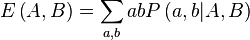
Correlation of observables X, Y is defined as

 represents the expected or average value of
This is a non-normalized form of the correlation coefficient considered in statistics (see Quantum correlation).
To formulate Bell's theorem, we formalize local realism as follows:
- There is a probability space
 and the observed outcomes by both Alice and Bob result by random sampling of the parameter
  .
. - The values observed by Alice or Bob are functions of the local detector settings and the hidden parameter only. Thus
- Value observed by Alice with detector setting
 is
is 
- Value observed by Bob with detector setting
 is
is 
- Value observed by Alice with detector setting
 has a probability measure
  and the expectation of a random variable X on with respect to is written
Bell's inequality. The CHSH inequality (1) holds under the hidden variables assumptions above.
For simplicity, let us first assume the observed values are +1 or −1; we remove this assumption in Remark 1 below.
Let
. Then at least one of
![\begin{align}
&\quad A(a, \lambda) B(b, \lambda) + A(a, \lambda) B(b', \lambda) + A(a', \lambda) B(b, \lambda) - A(a', \lambda) \ B(b', \lambda)\\
&= A(a, \lambda) \left[B(b, \lambda) + B(b', \lambda)\right] + A(a', \lambda) \left[B(b, \lambda) - B(b', \lambda)\right]\\
&\leq 2
\end{align}](http://upload.wikimedia.org/math/6/b/0/6b0c71af0675a049a021ce15aa7a4353.png)
![\begin{align}
&\quad \mathbf{C}(A(a), B(b)) + \mathbf{C}(A(a), B(b')) +
\mathbf{C}(A(a'), B(b)) - \mathbf{C}(A(a'), B(b'))&\\
&= \int_\Lambda A(a, \lambda) B(b, \lambda) \rho(\lambda) d \lambda +
\int_\Lambda A(a, \lambda) B(b', \lambda) \rho(\lambda) d \lambda +
\int_\Lambda A(a', \lambda) B(b, \lambda) \rho(\lambda) d \lambda -
\int_\Lambda A(a', \lambda) B(b', \lambda) \rho(\lambda) d \lambda&\\
&= \int_\Lambda \big\{
A(a, \lambda) B(b, \lambda) +
A(a, \lambda) B(b', \lambda) +
A(a', \lambda) B(b, \lambda) -
A(a', \lambda) B(b', \lambda)
\big\} \rho(\lambda) d \lambda&\\
&= \int_\Lambda \big\{
A(a, \lambda) \left[
B(b, \lambda) + B(b', \lambda)
\right] + A(a', \lambda) \left[
B(b, \lambda) - B(b', \lambda)
\right]
\big\} \rho(\lambda) d \lambda\\
&\leq 2
\end{align}](http://upload.wikimedia.org/math/e/f/b/efb4e7b856121a51e344816fdd072423.png)
- Remark 1
 ,
,  are allowed to take on any real values between −1 and +1. Indeed, the relevant idea is that each summand in the above average is bounded above by 2. This is easily seen as true in the more general case:
![\begin{align}
&\quad A(a, \lambda) B(b, \lambda) + A(a, \lambda) B(b', \lambda) + A(a', \lambda) B(b, \lambda) - A(a', \lambda) B(b', \lambda)\\
&= A(a, \lambda) \left[B(b, \lambda) + B(b', \lambda)\right] + A(a', \lambda) \left[B(b, \lambda) - B(b', \lambda)\right]\\
&\leq \big| A(a, \lambda) \left[B(b, \lambda) + B(b', \lambda)\right] + A(a', \lambda) \left[B(b, \lambda) - B(b', \lambda)\right] \big|\\
&\leq \big| A(a, \lambda) \left[B(b, \lambda) + B(b', \lambda)\right] \big| + \big| A(a', \lambda) \left[B(b, \lambda) - B(b', \lambda)\right] \big|\\
&\leq \big| B(b, \lambda) + B(b', \lambda) \big| + \big| B(b, \lambda) - B(b', \lambda) \big| \leq 2
\end{align}](http://upload.wikimedia.org/math/8/d/b/8db6d00da019a6286a644943a1661449.png)


- Remark 2
 in Bell's original proof is associated with the source and is shared by Alice and Bob, there may be others that are associated with the separate detectors, these others being conditionally independent given the first, and with conditional probability distributions only depending on the corresponding local setting (if dependent on the settings at all). This argument was used by Bell in 1971, and again by Clauser and Horne in 1974,[13] to justify a generalisation of the theorem forced on them by the real experiments, in which detectors were never 100% efficient. The derivations were given in terms of the averages of the outcomes over the local detector variables. The formalisation of local realism was thus effectively changed, replacing A and B by averages and retaining the symbol but with a slightly different meaning. It was henceforth restricted (in most theoretical work) to mean only those components that were associated with the source.
However, with the extension proved in Remark 1, CHSH inequality still holds even if the instruments themselves contain hidden variables. In that case, averaging over the instrument hidden variables gives new variables:
 , which still have values in the range [−1, +1] to which we can apply the previous result.
[edit] Bell inequalities are violated by quantum mechanical predictions
In the usual quantum mechanical formalism, the observables X and Y are represented as self-adjoint operators on a Hilbert space. To compute the correlation, assume that X and Y are represented by matrices in a finite dimensional space and that X and Y commute; this special case suffices for our purposes below. The von Neumann measurement postulate states: a series of measurements of an observable X on a series of identical systems in state produces a distribution of real values. By the assumption that observables are finite matrices, this distribution is discrete. The probability of observing λ is non-zero if and only if λ is an eigenvalue of the matrix X and moreover the probability is

 is
is

 be the spin singlet state for a pair of electrons discussed in the EPR paradox. This is a specially constructed state described by the following vector in the tensor product


 ,
,  correspond to Bob's spin measurements along x′ and z′. Note that the A operators commute with the B operators, so we can apply our calculation for the correlation. In this case, we can show that the CHSH inequality fails. In fact, a straightforward calculation shows that

 is indeed the upper bound for quantum mechanics called Tsirelson's bound. The operators giving this maximal value are always isomorphic to the Pauli matrices.
[edit] Practical experiments testing Bell's theorem

The source S produces pairs of "photons", sent in opposite directions. Each photon encounters a two-channel polariser whose orientation (a or b) can be set by the experimenter. Emerging signals from each channel are detected and coincidences of four types (++, −−, +− and −+) counted by the coincidence monitor.
Main article: Bell test experiments
Experimental tests can determine whether the Bell inequalities required by local realism hold up to the empirical evidence.Bell's inequalities are tested by "coincidence counts" from a Bell test experiment such as the optical one shown in the diagram. Pairs of particles are emitted as a result of a quantum process, analysed with respect to some key property such as polarisation direction, then detected. The setting (orientations) of the analysers are selected by the experimenter.
Bell test experiments to date overwhelmingly violate Bell's inequality. Indeed, a table of Bell test experiments performed prior to 1986 is given in 4.5 of Redhead, 1987.[17] Of the thirteen experiments listed, only two reached results contradictory to quantum mechanics; moreover, according to the same source, when the experiments were repeated, "the discrepancies with QM could not be reproduced".
Nevertheless, the issue is not conclusively settled. According to Shimony's 2004 Stanford Encyclopedia overview article:[5]
Most of the dozens of experiments performed so far have favored Quantum Mechanics, but not decisively because of the 'detection loopholes' or the 'communication loophole.' The latter has been nearly decisively blocked by a recent experiment and there is a good prospect for blocking the former.To explore the 'detection loophole', one must distinguish the classes of homogeneous and inhomogeneous Bell inequality.
The standard assumption in Quantum Optics is that "all photons of given frequency, direction and polarization are identical" so that photodetectors treat all incident photons on an equal basis. Such a fair sampling assumption generally goes unacknowledged, yet it effectively limits the range of local theories to those that conceive of the light field as corpuscular. The assumption excludes a large family of local realist theories, in particular, Max Planck's description. We must remember the cautionary words of Albert Einstein[18] shortly before he died: "Nowadays every Tom, Dick and Harry ('jeder Kerl' in German original) thinks he knows what a photon is, but he is mistaken".
Those who maintain the concept of duality, or simply of light being a wave, recognize the possibility or actuality that the emitted atomic light signals have a range of amplitudes and, furthermore, that the amplitudes are modified when the signal passes through analyzing devices such as polarizers and beam splitters. It follows that not all signals have the same detection probability.[19]
[edit] Two classes of Bell inequalities
The fair sampling problem was faced openly in the 1970s. In early designs of their 1973 experiment, Freedman and Clauser[20] used fair sampling in the form of the Clauser–Horne–Shimony–Holt (CHSH[16]) hypothesis. However, shortly afterwards Clauser and Horne[13] made the important distinction between inhomogeneous (IBI) and homogeneous (HBI) Bell inequalities. Testing an IBI requires that we compare certain coincidence rates in two separated detectors with the singles rates of the two detectors. Nobody needed to perform the experiment, because singles rates with all detectors in the 1970s were at least ten times all the coincidence rates. So, taking into account this low detector efficiency, the QM prediction actually satisfied the IBI. To arrive at an experimental design in which the QM prediction violates IBI we require detectors whose efficiency exceeds 82% for singlet states, but have very low dark rate and short dead and resolving times. This is well above the 30% achievable[21] so Shimony’s optimism in the Stanford Encyclopedia, quoted in the preceding section, appears over-stated.[edit] Practical challenges
Main article: Loopholes in Bell test experiments
Because detectors don't detect a large fraction of all photons, Clauser and Horne[13] recognized that testing Bell's inequality requires some extra assumptions. They introduced the No Enhancement Hypothesis (NEH):Given this assumption, there is a Bell inequality between the coincidence rates with polarizers and coincidence rates without polarizers.A light signal, originating in an atomic cascade for example, has a certain probability of activating a detector. Then, if a polarizer is interposed between the cascade and the detector, the detection probability cannot increase.
The experiment was performed by Freedman and Clauser,[20] who found that the Bell's inequality was violated. So the no-enhancement hypothesis cannot be true in a local hidden variables model. The Freedman–Clauser experiment reveals that local hidden variables imply the new phenomenon of signal enhancement:
This is perhaps not surprising, as it is known that adding noise to data can, in the presence of a threshold, help reveal hidden signals (this property is known[22] as stochastic resonance). One cannot conclude that this is the only local-realist alternative to Quantum Optics, but it does show that the word loophole is biased. Moreover, the analysis leads us to recognize that the Bell-inequality experiments, rather than showing a breakdown of realism or locality, are capable of revealing important new phenomena.In the total set of signals from an atomic cascade there is a subset whose detection probability increases as a result of passing through a linear polarizer.
[edit] Theoretical challenges
Most advocates of the hidden variables idea believe that experiments have ruled out local hidden variables. They are ready to give up locality, explaining the violation of Bell's inequality by means of a non-local hidden variable theory, in which the particles exchange information about their states. This is the basis of the Bohm interpretation of quantum mechanics, which requires that all particles in the universe be able to instantaneously exchange information with all others. A 2007 experiment ruled out a large class of non-Bohmian non-local hidden variable theories.[23]If the hidden variables can communicate with each other faster than light, Bell's inequality can easily be violated. Once one particle is measured, it can communicate the necessary correlations to the other particle. Since in relativity the notion of simultaneity is not absolute, this is unattractive. One idea is to replace instantaneous communication with a process that travels backwards in time along the past Light cone. This is the idea behind a transactional interpretation of quantum mechanics, which interprets the statistical emergence of a quantum history as a gradual coming to agreement between histories that go both forward and backward in time.[24]
A few advocates of deterministic models have not given up on local hidden variables. For example, Gerard 't Hooft has argued that the superdeterminism loophole cannot be dismissed.[25][26]
The quantum mechanical wavefunction can also provide a local realistic description, if the wavefunction values are interpreted as the fundamental quantities that describe reality. Such an approach is called a many-worlds interpretation of quantum mechanics. In this view, two distant observers both split into superpositions when measuring a spin. The Bell inequality violations are no longer counterintuitive, because it is not clear which copy of the observer B observer A will see when going to compare notes. If reality includes all the different outcomes, locality in physical space (not outcome space) places no restrictions on how the split observers can meet up.
This implies that there is a subtle assumption in the argument that realism is incompatible with quantum mechanics and locality. The assumption, in its weakest form, is called counterfactual definiteness. This states that if the results of an experiment are always observed to be definite, there is a quantity that determines what the outcome would have been even if you don't do the experiment.
Many worlds interpretations are not only counterfactually indefinite, they are factually indefinite. The results of all experiments, even ones that have been performed, are not uniquely determined.
E. T. Jaynes[27] pointed out two hidden assumptions in Bell Inequality that could limit its generality. According to him:
- Bell interpreted conditional probability P(X|Y) as a causal inference, i.e. Y exerted a causal inference on X in reality. However, P(X|Y) actually only means logical inference (deduction). Causes cannot travel faster than light or backward in time, but deduction can.
- Bell's inequality does not apply to some possible hidden variable theories. It only applies to a certain class of local hidden variable theories. In fact, it might have just missed the kind of hidden variable theories that Einstein is most interested in.
[edit] Final remarks
The violations of Bell's inequalities, due to quantum entanglement, just provide the definite demonstration of something that was already strongly suspected, that quantum physics cannot be represented by any version of the classical picture of physics.[28] Some earlier elements that had seemed incompatible with classical pictures included apparent complementarity and (hypothesized) wavefunction collapse. Complementarity is now seen not as an independent ingredient of the quantum picture but rather as a direct consequence of the Quantum decoherence expected from the quantum formalism itself. The possibility of wavefunction collapse is now seen as one possible problematic ingredient of some interpretations, rather than as an essential part of quantum mechanics. The Bell violations show that no resolution of such issues can avoid the ultimate strangeness of quantum behavior.[29]The EPR paper "pinpointed" the unusual properties of the entangled states, e.g. the above-mentioned singlet state, which is the foundation for present-day applications of quantum physics, such as quantum cryptography; one application involves the measurement of quantum entanglement as a physical source of bits for Rabin's oblivious transfer protocol. This strange non-locality was originally supposed to be a Reductio ad absurdum, because the standard interpretation could easily do away with action-at-a-distance by simply assigning to each particle definite spin-states. Bell's theorem showed that the "entangledness" prediction of quantum mechanics has a degree of non-locality that cannot be explained away by any local theory.
In well-defined Bell experiments (see the paragraph on "test experiments") one can now falsify either quantum mechanics or Einstein's quasi-classical assumptions: currently many experiments of this kind have been performed, and the experimental results support quantum mechanics, though some believe that detectors give a biased sample of photons, so that until nearly every photon pair generated is observed there will be loopholes.
What is powerful about Bell's theorem is that it doesn't refer to any particular physical theory. What makes Bell's theorem unique and powerful is that it shows that nature violates the most general assumptions behind classical pictures, not just details of some particular models. No combination of local deterministic and local random variables can reproduce the phenomena predicted by quantum mechanics and repeatedly observed in experiments.[30]
[edit] See also
- Bell test experiments
- Bohr–Einstein debates on quantum mechanics
- CHSH Bell test
- Counterfactual definiteness
- Fundamental Fysiks Group
- GHZ experiment
- Hidden variable theory
- Local hidden variable theory
- Loopholes in Bell test experiments
- Leggett inequality
- Leggett–Garg inequality
- Measurement in quantum mechanics
- Mott problem
- Quantum entanglement
- Quantum mechanical Bell test prediction
- Renninger negative-result experiment
[edit] Notes
- ^ a b C.B. Parker (1994). McGraw Hill Encyclopaedia of Physics (2nd ed.). McGraw Hill. p. 542. ISBN 0-07-051400-3.
- ^ C.B. Parker (1994). McGraw Hill Encyclopaedia of Physics (2nd ed.). McGraw Hill. p. 541. ISBN 0-07-051400-3.
- ^ a b c d e f g Bell, John (1964). "On the Einstein Podolsky Rosen Paradox". Physics 1 (3): 195–200. http://www.drchinese.com/David/Bell_Compact.pdf.
- ^ Bohm, David Quantum Theory. Prentice−Hall, 1951.
- ^ a b c d Article on Bell's Theorem by Abner Shimony in the Stanford Encyclopedia of Philosophy, (2004).
- ^ Leggett, Anthony (2003). "Nonlocal Hidden-Variable Theories and Quantum Mechanics: An Incompatibility Theorem". Foundations of Physics 33 (10): 1469–1493.
- ^ Griffiths, David J. (1998). Introduction to Quantum Mechanics (2nd ed.). Pearson/Prentice Hall. pp. 423.
- ^ Merzbacher, Eugene (2005). Quantum Mechanics (3rd ed.). John Wiley & Sons. pp. 18, 362.
- ^ Stapp, 1975
- ^ Bell, JS, "On the impossible pilot wave." Foundations of Physics (1982) 12:989–99. Reprinted in Speakable and unspeakable in quantum mechanics: collected papers on quantum philosophy. CUP, 2004, p. 160.
- ^ Bell, JS, "On the impossible pilot wave." Foundations of Physics (1982) 12:989–99. Reprinted in Speakable and unspeakable in quantum mechanics: collected papers on quantum philosophy. CUP, 2004, p. 161.
- ^ Einstein, A.; Podolsky, B.; Rosen, N. (1935). "Can Quantum-Mechanical Description of Physical Reality Be Considered Complete?". Physical Review 47 (10): 777. Bibcode 1935PhRv...47..777E. doi:10.1103/PhysRev.47.777.
- ^ a b c d Clauser, John F. (1974). "Experimental consequences of objective local theories". Physical Review D 10 (2): 526. Bibcode 1974PhRvD..10..526C. doi:10.1103/PhysRevD.10.526.
- ^ Eberhard, P. H. (1977). "Bell's theorem without hidden variables". Nuovo Cimento B 38: 75–80. Bibcode 1977NCimB..38...75E. doi:10.1007/BF02726212.
- ^ Bell, JS, Speakable and unspeakable in quantum mechanics: Introduction remarks at Naples–Amalfi meeting., 1984. Reprinted in Speakable and unspeakable in quantum mechanics: collected papers on quantum philosophy. CUP, 2004, p. 29.
- ^ a b c Clauser, John; Horne, Michael; Shimony, Abner; Holt, Richard (1969). "Proposed Experiment to Test Local Hidden-Variable Theories". Physical Review Letters 23 (15): 880. Bibcode 1969PhRvL..23..880C. doi:10.1103/PhysRevLett.23.880.
- ^ M. Redhead, Incompleteness, Nonlocality and Realism, Clarendon Press (1987)
- ^ A. Einstein in Correspondance Einstein–Besso, p.265 (Herman, Paris, 1979)
- ^ Marshall and Santos, Semiclassical optics as an alternative to nonlocality Recent Research Developments in Optics 2:683–717 (2002) ISBN 81-7736-140-6
- ^ a b Freedman, Stuart J.; Clauser, John F. (1972). "Experimental Test of Local Hidden-Variable Theories". Physical Review Letters 28 (14): 938. Bibcode 1972PhRvL..28..938F. doi:10.1103/PhysRevLett.28.938.
- ^ Giorgio Brida; Marco Genovese; Marco Gramegna; Fabrizio Piacentini; Enrico Predazzi; Ivano Ruo-Berchera (2007). "Experimental tests of hidden variable theories from dBB to Stochastic Electrodynamics". Journal of Physics: Conference Series 67 (12047): 012047. arXiv:quant-ph/0612075. Bibcode 2007JPhCS..67a2047G. doi:10.1088/1742-6596/67/1/012047.
- ^ Gammaitoni, Luca; Hänggi, Peter; Jung, Peter; Marchesoni, Fabio (1998). "Stochastic resonance". Reviews of Modern Physics 70: 223. Bibcode 1998RvMP...70..223G. doi:10.1103/RevModPhys.70.223.
- ^ Gröblacher, Simon; Paterek, Tomasz; Kaltenbaek, Rainer; Brukner, Časlav; Żukowski, Marek; Aspelmeyer, Markus; Zeilinger, Anton (2007). "An experimental test of non-local realism". Nature 446 (7138): 871–5. arXiv:0704.2529. Bibcode 2007Natur.446..871G. doi:10.1038/nature05677. PMID 17443179.
- ^ Cramer, John (1986). "The transactional interpretation of quantum mechanics". Reviews of Modern Physics 58 (3): 647. Bibcode 1986RvMP...58..647C. doi:10.1103/RevModPhys.58.647.
- ^ Gerard 't Hooft (2009). "Entangled quantum states in a local deterministic theory". arXiv:0908.3408 [quant-ph].
- ^ Gerard 't Hooft (2007). "The Free-Will Postulate in Quantum Mechanics". arXiv:quant-ph/0701097 [quant-ph].
- ^ Jaynes, E. T. (1989). "Clearing up Mysteries—The Original Goal". Maximum Entropy and Bayesian Methods: 12. http://bayes.wustl.edu/etj/articles/cmystery.pdf.
- ^ Roger Penrose (2007). The Road to Reality. Vintage books. p. 583. ISBN 0-679-77631-1.
- ^ E. Abers (2004). Quantum Mechanics. Addison Wesley. pp. 193–195. ISBN 9780131461000.
- ^ R.G. Lerner, G.L. Trigg (1991). Encyclopaedia of Physics (2nd ed.). VHC publishers. p. 495. ISBN 3-527-26954-1 (Verlagsgesellschaft) 0-89573-752-3 (VHC Inc.).
[edit] References
- A. Aspect et al., Experimental Tests of Realistic Local Theories via Bell's Theorem, Phys. Rev. Lett. 47, 460 (1981)
- A. Aspect et al., Experimental Realization of Einstein–Podolsky–Rosen–Bohm Gedankenexperiment: A New Violation of Bell's Inequalities, Phys. Rev. Lett. 49, 91 (1982).
- A. Aspect et al., Experimental Test of Bell's Inequalities Using Time-Varying Analyzers, Phys. Rev. Lett. 49, 1804 (1982).
- A. Aspect and P. Grangier, About resonant scattering and other hypothetical effects in the Orsay atomic-cascade experiment tests of Bell inequalities: a discussion and some new experimental data, Lettere al Nuovo Cimento 43, 345 (1985)
- B. D'Espagnat, The Quantum Theory and Reality, Scientific American, 241, 158 (1979)
- J. S. Bell, On the problem of hidden variables in quantum mechanics, Rev. Mod. Phys. 38, 447 (1966)
- J. S. Bell, On the Einstein Podolsky Rosen Paradox, Physics 1, 3, 195–200 (1964)
- J. S. Bell, Introduction to the hidden variable question, Proceedings of the International School of Physics 'Enrico Fermi', Course IL, Foundations of Quantum Mechanics (1971) 171–81
- J. S. Bell, Bertlmann’s socks and the nature of reality, Journal de Physique, Colloque C2, suppl. au numero 3, Tome 42 (1981) pp C2 41–61
- J. S. Bell, Speakable and Unspeakable in Quantum Mechanics (Cambridge University Press 1987) [A collection of Bell's papers, including all of the above.]
- J. F. Clauser and A. Shimony, Bell's theorem: experimental tests and implications, Reports on Progress in Physics 41, 1881 (1978)
- J. F. Clauser and M. A. Horne, Phys. Rev D 10, 526–535 (1974)
- E. S. Fry, T. Walther and S. Li, Proposal for a loophole-free test of the Bell inequalities, Phys. Rev. A 52, 4381 (1995)
- E. S. Fry, and T. Walther, Atom based tests of the Bell Inequalities — the legacy of John Bell continues, pp 103–117 of Quantum [Un]speakables, R.A. Bertlmann and A. Zeilinger (eds.) (Springer, Berlin-Heidelberg-New York, 2002)
- R. B. Griffiths, Consistent Quantum Theory', Cambridge University Press (2002).
- L. Hardy, Nonlocality for 2 particles without inequalities for almost all entangled states. Physical Review Letters 71 (11) 1665–1668 (1993)
- M. A. Nielsen and I. L. Chuang, Quantum Computation and Quantum Information, Cambridge University Press (2000)
- P. Pearle, Hidden-Variable Example Based upon Data Rejection, Physical Review D 2, 1418–25 (1970)
- A. Peres, Quantum Theory: Concepts and Methods, Kluwer, Dordrecht, 1993.
- P. Pluch, Theory of Quantum Probability, PhD Thesis, University of Klagenfurt, 2006.
- B. C. van Frassen, Quantum Mechanics, Clarendon Press, 1991.
- M.A. Rowe, D. Kielpinski, V. Meyer, C.A. Sackett, W.M. Itano, C. Monroe, and D.J. Wineland, Experimental violation of Bell's inequalities with efficient detection,(Nature, 409, 791–794, 2001).
- S. Sulcs, The Nature of Light and Twentieth Century Experimental Physics, Foundations of Science 8, 365–391 (2003)
- S. Gröblacher et al., An experimental test of non-local realism,(Nature, 446, 871–875, 2007).
- D. N. Matsukevich, P. Maunz, D. L. Moehring, S. Olmschenk, and C. Monroe, Bell Inequality Violation with Two Remote Atomic Qubits, Phys. Rev. Lett. 100, 150404 (2008).
- The comic Dilbert, by Scott Adams, refers to Bell's Theorem in the 1992-09-21 and 1992-09-22 strips.
[edit] Further reading
The following are intended for general audiences.- Amir D. Aczel, Entanglement: The greatest mystery in physics (Four Walls Eight Windows, New York, 2001).
- A. Afriat and F. Selleri, The Einstein, Podolsky and Rosen Paradox (Plenum Press, New York and London, 1999)
- J. Baggott, The Meaning of Quantum Theory (Oxford University Press, 1992)
- N. David Mermin, "Is the moon there when nobody looks? Reality and the quantum theory", in Physics Today, April 1985, pp. 38–47.
- Louisa Gilder, The Age of Entanglement: When Quantum Physics Was Reborn (New York: Alfred A. Knopf, 2008)
- Brian Greene, The Fabric of the Cosmos (Vintage, 2004, ISBN 0-375-72720-5)
- Nick Herbert, Quantum Reality: Beyond the New Physics (Anchor, 1987, ISBN 0-385-23569-0)
- D. Wick, The infamous boundary: seven decades of controversy in quantum physics (Birkhauser, Boston 1995)
- R. Anton Wilson, Prometheus Rising (New Falcon Publications, 1997, ISBN 1-56184-056-4)
- Gary Zukav "The Dancing Wu Li Masters" (Perennial Classics, 2001, ISBN 0-06-095968-1)
[edit] External links
- An explanation of Bell's Theorem, based on N. D. Mermin's article, Mermin, N. D. (1981). "Bringing home the atomic world: Quantum mysteries for anybody". American Journal of Physics 49 (10): 940. Bibcode 1981AmJPh..49..940M. doi:10.1119/1.12594.
- Mermin: Spooky Actions At A Distance? Oppenheimer Lecture
- Quantum Entanglement Includes a simple explanation of Bell's Inequality.
- Bell's theorem on arXiv.org
- Interactive experiments with single photons: entanglement and Bell´s theorem
- Bell's Inequalities: Obscurantist Obfuscation or Condign Confabulation?


No comments:
Post a Comment